文字 1
SCHNEEBERGER
SCHNEEBERGER
5
Accessories
5.1 Extensions
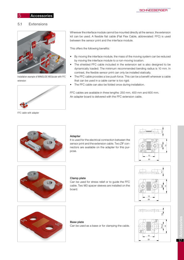
Wherever the interface module cannot be mounted directly at the sensor, the extension kit can be used. A flexible flat cable (Flat Flex Cable, abbreviated: FFC) is used between the sensor print and the interface module.
This offers the following benefits:
- By moving the interface module, the mass of the moving system can be reduced by moving the interface module to a non-moving location.
- The shielded FFC cable included in the extension set is also designed to be dynamically loaded. The minimum recommended bending radius is 10 mm. In contrast, the flexible sensor print can only be installed statically.
- The FFC cable provides a low push force. This can be a benefit wherever a cable that can be used in a cable carrier is too rigid.
- The FFC cable can also be folded once during installation.
Installation example of MINISLIDE MSQscale with FFC extension
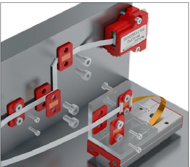
FFC cables are available in three lengths: 250 mm, 400 mm and 600 mm. An adapter board is delivered with the FFC extension cable.
FFC cable with adapter
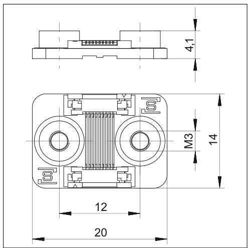
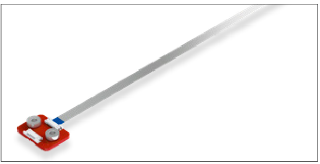
Adapter
It is used for the electrical connection between the sensor print and the extension cable. Two ZIF connectors are available on the adapter for this purpose.
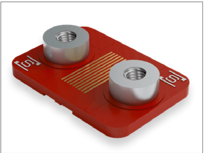
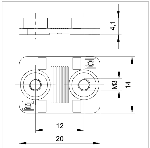
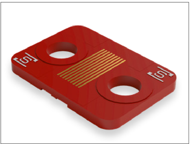
Clamp plate
Can be used for stress relief or to guide the FFC cable. Two M3 spacer sleeves are installed on the board.
Accessories
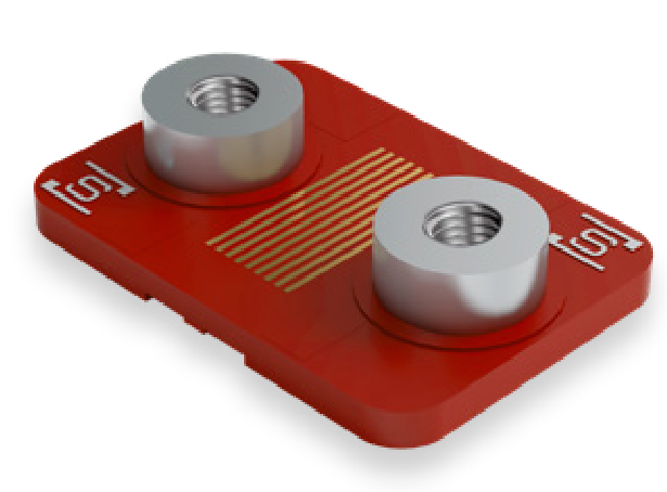
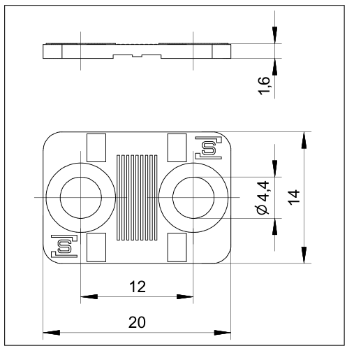
Base plate
Can be used as a base or for clamping the cable.
17

5 Accessories
SCHNEEBERGER
5.2 MINISLIDE MSQscale Counter and Position Indicator
For simple applications, experimental or prototype setups, we recommend the USB counters from Heilig & Schwab GmbH & Co. KG. The following counters can be ordered directly from Heilig & Schwab GmbH & Co. KG (www.heilig-schwab.de).
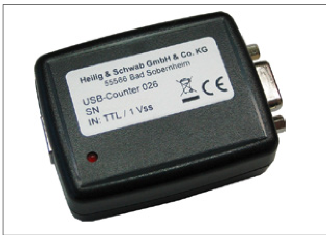
1-axis USB Counter
5.2.1. 1-axis USB Counter
The USB counter allows a MINISCALE PLUS or similar incremental encoder with TTL, 1 Vpp, or 11 µAss signal output to be connected directly to a computer using a USB interface.
With the included driver software, the USB counter can be quickly and easily integrated into your application.
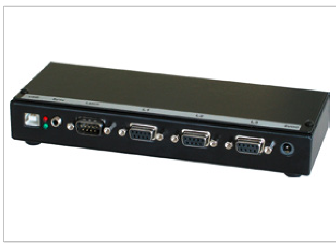
3-axis USB Counter
5.2.2. 3-axis USB Counter
The USB counter allows three MINISCALE PLUS or similar incremental encoders with TTL, or 1 Vpp signal output to be connected directly to a computer using a USB interface. Every counter input additionally has a latch signal input at its disposal.
With the included driver software, the USB counter can be quickly and easily integrated into your application.
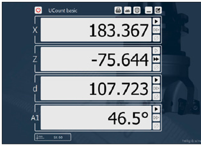
Digital display program "UCount basic"
5.2.3. "UCount basic" Digital Display Program
UCount basic is a digital display program for the evaluation of linear and angle sensors, which are connected to a computer (PC, laptop or tablet) via USB counters from Heilig & Schwab GmbH & Co. KG. Alternatively, the counters can also be connected to the computer via WLAN.
- Simple operation and clear presentation of all functions
- Meter display of up to 9 signal inputs
- Meter stop function
- Audible meter monitoring (threshold value)
- Calculation functions (addition, subtraction)
- Measuring functions (spacing, angle, included angle, radius)
- Correction function (linear correction, step-by-step (SBS) correction, parallelism correction)
- Reference point administration
- Expandable based on customer preference
System requirements:
- PC, laptop or tablet
- Windows Operating System, 32 or 64-bit version
- USB or WLAN interface
18
SCHNEEBERGER
6 Dimension Tables, Load Capacities, Weights and Moment Loads
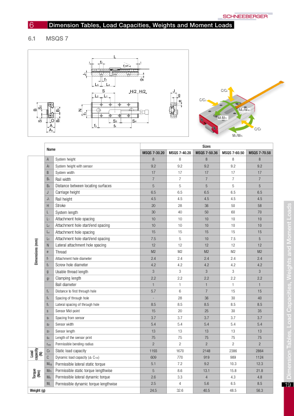
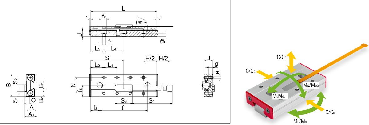
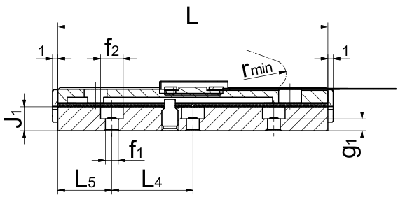
6.1 MSQS 7
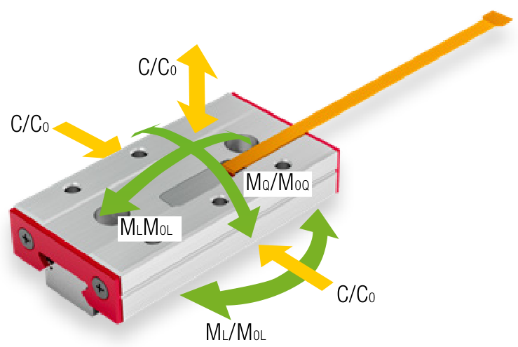
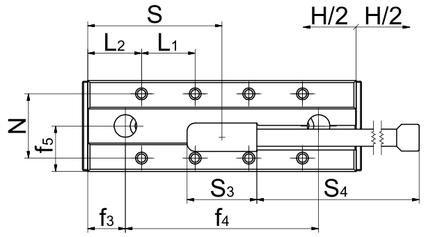
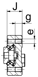
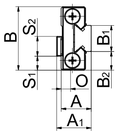
| Name | Sizes | ||||||
|---|---|---|---|---|---|---|---|
| MSQS 7-30.20 | MSQS 7-40.28 | MSQS 7-50.36 | MSQS 7-60.50 | MSQS 7-70.58 | |||
| Dimensions (mm) | A | System height | 8 | 8 | 8 | 8 | 8 |
| A1 | System height with sensor | 9.2 | 9.2 | 9.2 | 9.2 | 9.2 | |
| B | System width | 17 | 17 | 17 | 17 | 17 | |
| B1 | Rail width | 7 | 7 | 7 | 7 | 7 | |
| B2 | Distance between locating surfaces | 5 | 5 | 5 | 5 | 5 | |
| J | Carriage height | 6.5 | 6.5 | 6.5 | 6.5 | 6.5 | |
| J1 | Rail height | 4.5 | 4.5 | 4.5 | 4.5 | 4.5 | |
| H | Stroke | 20 | 28 | 36 | 50 | 58 | |
| L | System length | 30 | 40 | 50 | 60 | 70 | |
| L1 | Attachment hole spacing | 10 | 10 | 10 | 10 | 10 | |
| L2 | Attachment hole start/end spacing | 10 | 10 | 10 | 10 | 10 | |
| L4 | Attachment hole spacing | 15 | 15 | 15 | 15 | 15 | |
| L5 | Attachment hole start/end spacing | 7.5 | 5 | 10 | 7.5 | 5 | |
| N | Lateral attachment hole spacing | 12 | 12 | 12 | 12 | 12 | |
| e | Thread | M2 | M2 | M2 | M2 | M2 | |
| f1 | Attachment hole diameter | 2.4 | 2.4 | 2.4 | 2.4 | 2.4 | |
| f2 | Screw hole diameter | 4.2 | 4.2 | 4.2 | 4.2 | 4.2 | |
| g | Usable thread length | 3 | 3 | 3 | 3 | 3 | |
| g1 | Clamping length | 2.2 | 2.2 | 2.2 | 2.2 | 2.2 | |
| Ball diameter | 1 | 1 | 1 | 1 | 1 | ||
| f3 | Distance to first through hole | 5.7 | 6 | 7 | 15 | 15 | |
| f4 | Spacing of through hole | - | 28 | 36 | 30 | 40 | |
| f5 | Lateral spacing of through hole | 8.5 | 8.5 | 8.5 | 8.5 | 8.5 | |
| s | Sensor Mid-point | 15 | 20 | 25 | 30 | 35 | |
| S1 | Spacing from sensor | 3.7 | 3.7 | 3.7 | 3.7 | 3.7 | |
| S2 | Sensor width | 5.4 | 5.4 | 5.4 | 5.4 | 5.4 | |
| S3 | Sensor length | 13 | 13 | 13 | 13 | 13 | |
| S4 | Length of the sensor print | 75 | 75 | 75 | 75 | 75 | |
| rmin | Permissible bending radius | 2 | 2 | 2 | 2 | 2 | |
| Load capacity (N) | C0 | Static load capacity | 1193 | 1670 | 2148 | 2386 | 2864 |
| C | Dynamic load capacity (≙ C100) | 609 | 770 | 919 | 989 | 1124 | |
| Torque (Nm) | M0Q | Permissible lateral static torque | 5.1 | 7.2 | 9.2 | 10.3 | 12.3 |
| M0L | Permissible static torque lengthwise | 5 | 8.6 | 13.1 | 15.8 | 21.8 | |
| MQ | Permissible lateral dynamic torque | 2.6 | 3.3 | 4 | 4.3 | 4.8 | |
| ML | Permissible dynamic torque lengthwise | 2.5 | 4 | 5.6 | 6.5 | 8.5 | |
| Weight (g) | 24.5 | 32.6 | 40.5 | 48.5 | 56.3 | ||
Dimension Tables, Load Capacities, Weights and Moment Loads
19
SCHNEEBERGER
6 Dimension Tables, Load Capacities, Weights and Moment Loads
6.2 MSQS 9
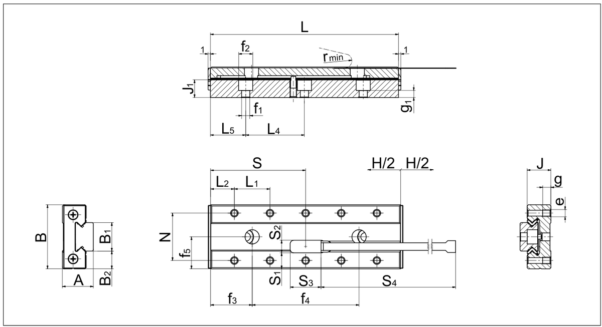
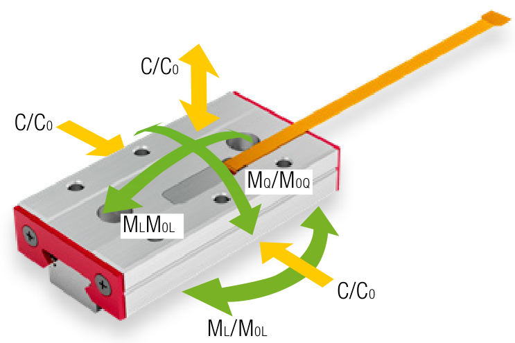
| Name | Sizes | ||||||
|---|---|---|---|---|---|---|---|
| MSQS 9-40.34 | MSQS 9-50.42 | MSQS 9-60.50 | MSQS 9-70.58 | MSQS 9-80.66 | |||
| Dimensions (mm) | A | System height | 10 | 10 | 10 | 10 | 10 |
| B | System width | 20 | 20 | 20 | 20 | 20 | |
| B1 | Rail width | 9 | 9 | 9 | 9 | 9 | |
| B2 | Distance between locating surfaces | 5.5 | 5.5 | 5.5 | 5.5 | 5.5 | |
| J | Carriage height | 8 | 8 | 8 | 8 | 8 | |
| J1 | Rail height | 5.5 | 5.5 | 5.5 | 5.5 | 5.5 | |
| H | Stroke | 34 | 42 | 50 | 58 | 66 | |
| L | System length | 40 | 50 | 60 | 70 | 80 | |
| L1 | Attachment hole spacing | 10 | 10 | 10 | 10 | 10 | |
| L2 | Attachment hole start/end spacing | 10 | 10 | 10 | 10 | 10 | |
| L4 | Attachment hole spacing | 20 | 20 | 20 | 20 | 20 | |
| L5 | Attachment hole start/end spacing | 10 | 5 | 10 | 5 | 10 | |
| N | Lateral attachment hole spacing | 15 | 15 | 15 | 15 | 15 | |
| e | Thread | M3 | M3 | M3 | M3 | M3 | |
| f1 | Attachment hole diameter | 3.5 | 3.5 | 3.5 | 3.5 | 3.5 | |
| f2 | Screw hole diameter | 6 | 6 | 6 | 6 | 6 | |
| g | Usable thread length | 3 | 3 | 3 | 3 | 3 | |
| g1 | Clamping length | 2 | 2 | 2 | 2 | 2 | |
| Ball diameter | 1 | 1 | 1 | 1 | 1 | ||
| f3 | Distance to first through hole | 10 | 10 | 15 | 15 | 15 | |
| f4 | Spacing of through hole | - | 30 | 30 | 40 | 50 | |
| f5 | Lateral spacing of through hole | 10 | 10 | 10 | 10 | 10 | |
| s | Sensor Mid-point | 20 | 25 | 30 | 35 | 40 | |
| S1 | Spacing from sensor | 4.2 | 4.2 | 4.2 | 4.2 | 4.2 | |
| S2 | Sensor width | 5.4 | 5.4 | 5.4 | 5.4 | 5.4 | |
| S3 | Sensor length | 13 | 13 | 13 | 13 | 13 | |
| S4 | Length of the sensor print | 75 | 75 | 75 | 75 | 75 | |
| rmin | Permissible bending radius | 2 | 2 | 2 | 2 | 2 | |
| Load capacity (N) | C0 | Static load capacity | 1432 | 1909 | 2386 | 2864 | 3341 |
| C | Dynamic load capacity (≙ C100) | 692 | 846 | 989 | 1124 | 1252 | |
| Torque (Nm) | M0Q | Permissible lateral static torque | 7.6 | 10.1 | 12.6 | 15.2 | 17.7 |
| M0L | Permissible static torque lengthwise | 6.7 | 10.8 | 15.8 | 21.8 | 28.7 | |
| MQ | Permissible lateral dynamic torque | 3.7 | 4.5 | 5.2 | 6 | 6.6 | |
| ML | Permissible dynamic torque lengthwise | 3.2 | 4.8 | 6.5 | 8.5 | 10.7 | |
| Weight (g) | 45.6 | 56.9 | 68.1 | 79.2 | 90.3 | ||
SCHNEEBERGER
6 Dimension Tables, Load Capacities, Weights and Moment Loads
6.3 MSQS 12
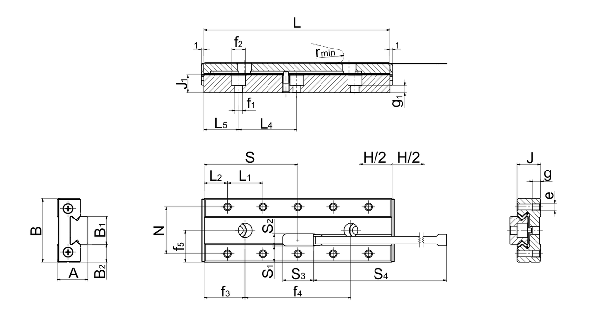
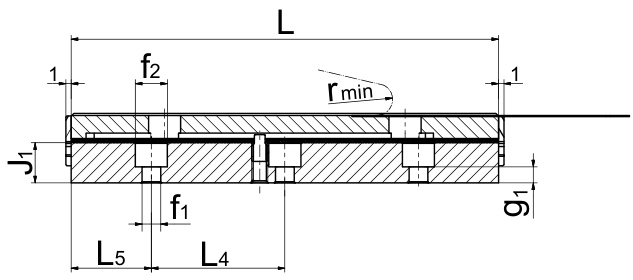
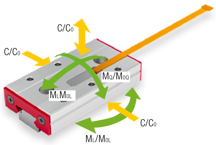
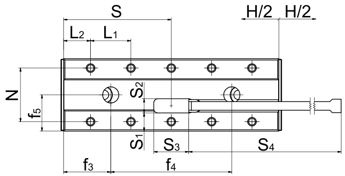
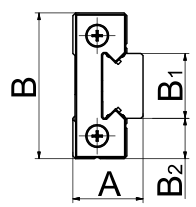
| Name | Name | Sizes | |||||
|---|---|---|---|---|---|---|---|
| MSQS 12-50.45 | MSQS 12-80.63 | MSQS 12-100.70 | MSQS 12-100.70 | ||||
| Dimensions (mm) | A | System height | 13 | 13 | 13 | 13 | |
| B | System width | 27 | 27 | 27 | 27 | ||
| B1 | Rail width | 12 | 12 | 12 | 12 | ||
| B2 | Distance between locating surfaces | 7.5 | 7.5 | 7.5 | 7.5 | ||
| J | Carriage height | 10 | 10 | 10 | 10 | ||
| J1 | Rail height | 7.5 | 7.5 | 7.5 | 7.5 | ||
| H | Stroke | 45 | 48 | 63 | 70 | ||
| L | System length | 50 | 60 | 80 | 100 | ||
| L1 | Attachment hole spacing | 15 | 15 | 15 | 15 | ||
| L2 | Attachment hole start/end spacing | 10 | 7.5 | 10 | 12.5 | ||
| L4 | Attachment hole spacing | 25 | 25 | 25 | 25 | ||
| L5 | Attachment hole start/end spacing | 12.5 | 5 | 15 | 12.5 | ||
| N | Lateral attachment hole spacing | 20 | 20 | 20 | 20 | ||
| e | Thread | M3 | M3 | M3 | M3 | ||
| f1 | Attachment hole diameter | 3.5 | 3.5 | 3.5 | 3.5 | ||
| f2 | Screw hole diameter | 6 | 6 | 6 | 6 | ||
| g | Usable thread length | 3.5 | 3.5 | 3.5 | 3.5 | ||
| g1 | Clamping length | 3 | 3 | 3 | 3 | ||
| Ball diameter | 1.5 | 1.5 | 1.5 | 1.5 | |||
| f3 | Distance to first through hole | 10 | 15 | 17.5 | 20 | ||
| f4 | Spacing of through hole | 30 | 30 | 45 | 60 | ||
| f5 | Lateral spacing of through hole | 13.5 | 13.5 | 13.5 | 13.5 | ||
| s | Sensor Mid-point | 25 | 30 | 40 | 50 | ||
| S1 | Spacing from sensor | 6.7 | 6.7 | 6.7 | 6.7 | ||
| S2 | Sensor width | 5.4 | 5.4 | 5.4 | 5.4 | ||
| S3 | Sensor length | 13 | 13 | 13 | 13 | ||
| S4 | Length of the sensor print | 75 | 75 | 75 | 75 | ||
| rmin | Permissible bending radius | 2 | 2 | 2 | 2 | ||
| Load capacity (N) | C0 | Static load capacity | 2685 | 3759 | 5370 | 7518 | |
| C | Dynamic load capacity (≙ C100) | 1427 | 1806 | 2318 | 2934 | ||
| Torque (Nm) | M0Q | Permissible lateral static torque | 18.9 | 26.5 | 37.9 | 53 | |
| M0L | Permissible static torque lengthwise | 15.7 | 27 | 49.5 | 90.1 | ||
| M0 | Permissible lateral dynamic torque | 10.1 | 12.7 | 16.3 | 20.7 | ||
| ML | Permissible dynamic torque lengthwise | 8.3 | 12.9 | 21.4 | 35.1 | ||
| Weight (g) | Weight (g) | 103.9 | 124.4 | 165.5 | 206.5 | ||
Dimension Tables, Load Capacities, Weights and Moment Loads
21
SCHNEEBERGER
6 Dimension Tables, Load Capacities, Weights and Moment Loads
6.4 MSQS 15
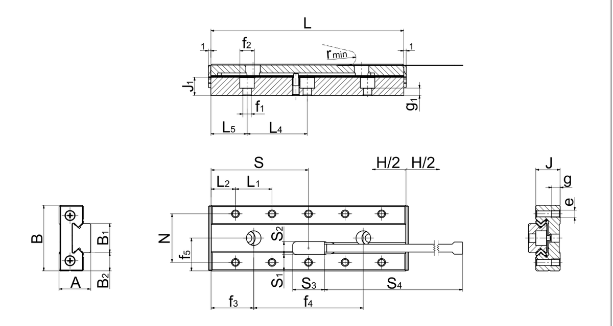
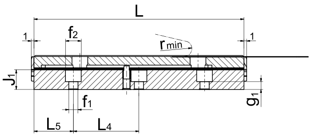
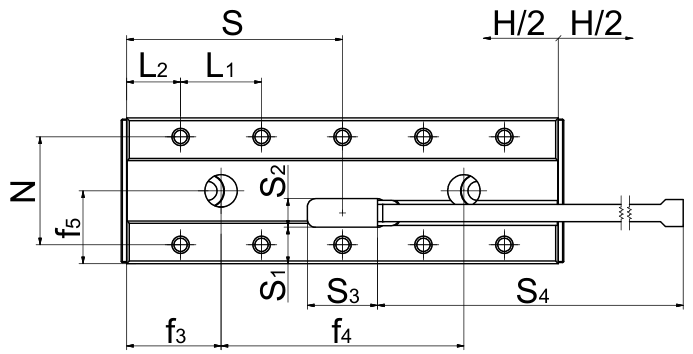
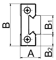
| Name | Sizes | |||||
|---|---|---|---|---|---|---|
| MSQS 15-70.66 | MSQS 15-90.70 | MSQS 15-110.96 | MSQS 15-130.102 | |||
| Dimensions (mm) | A | System height | 16 | 16 | 16 | 16 |
| B | System width | 32 | 32 | 32 | 32 | |
| B1 | Rail width | 15 | 15 | 15 | 15 | |
| B2 | Distance between locating surfaces | 8.5 | 8.5 | 8.5 | 8.5 | |
| J | Carriage height | 12 | 12 | 12 | 12 | |
| J1 | Rail height | 9.5 | 9.5 | 9.5 | 9.5 | |
| H | Stroke | 66 | 70 | 96 | 102 | |
| L | System length | 70 | 90 | 110 | 130 | |
| L1 | Attachment hole spacing | 20 | 20 | 20 | 20 | |
| L2 | Attachment hole start/end spacing | 15 | 15 | 15 | 15 | |
| L4 | Attachment hole spacing | 40 | 40 | 40 | 40 | |
| L5 | Attachment hole start/end spacing | 15 | 5 | 15 | 5 | |
| N | Lateral attachment hole spacing | 25 | 25 | 25 | 25 | |
| e | Thread | M3 | M3 | M3 | M3 | |
| f1 | Attachment hole diameter | 3.5 | 3.5 | 3.5 | 3.5 | |
| f2 | Screw hole diameter | 6 | 6 | 6 | 6 | |
| g | Usable thread length | 4 | 4 | 4 | 4 | |
| g1 | Clamping length | 5 | 5 | 5 | 5 | |
| Ball diameter | 2 | 2 | 2 | 2 | ||
| f3 | Distance to first through hole | 15 | 25 | 25 | 25 | |
| f4 | Spacing of through hole | 40 | 40 | 60 | 80 | |
| f5 | Lateral spacing of through hole | 16 | 16 | 16 | 16 | |
| s | Sensor Mid-point | 35 | 45 | 55 | 65 | |
| S1 | Spacing from sensor | 8.3 | 8.3 | 8.3 | 8.3 | |
| S2 | Sensor width | 5.4 | 5.4 | 5.4 | 5.4 | |
| S3 | Sensor length | 13 | 13 | 13 | 13 | |
| S4 | Length of the sensor print | 75 | 75 | 75 | 75 | |
| rmin | Permissible bending radius | 2 | 2 | 2 | 2 | |
| Load capacity (N) | C0 | Static load capacity | 4773 | 7637 | 8592 | 11456 |
| C | Dynamic load capacity (≙ C100) | 2611 | 3628 | 3940 | 4820 | |
| Torque (Nm) | M0Q | Permissible lateral static torque | 42.5 | 68 | 76.5 | 102 |
| M0L | Permissible static torque lengthwise | 36.7 | 80.9 | 99.5 | 166.6 | |
| MQ | Permissible lateral dynamic torque | 23.2 | 32.3 | 35.1 | 42.9 | |
| ML | Permissible dynamic torque lengthwise | 20.1 | 38.4 | 45.6 | 70.1 | |
| Weight (g) | 216.2 | 277.5 | 338.6 | 399.5 | ||
22
SCHNEEBERGER
7 Load Carrying Capacity and Service Life
7.1 Principles
The load capacities are based on the principles of DIN 636.
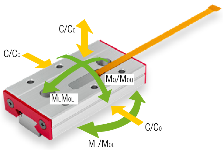
In accordance with DIN in most applications a permanent overall deformation of 0.0001 times the rolling element diameter can be permitted without adversely affecting the operating behaviour of the bearing. Consequently, the static load capacity C0 is set sufficiently high that the aforementioned deformation occurs approximately when the equivalent static load corresponds to the static load capacity. Being guided by the dynamic load capacity C is recommended so that the aforementioned overall deformation does not occur.
The dynamic load capacity C is the load at which a nominal service life L of 100 km of travel distance is achieved. It is important to note when calculating the service life that not only the load, which acts vertically on the guideway, should be taken into account but also the load spectrum of all acting forces and moments.
The service life corresponds to the total travel distance in meters which a guideway facilitates. And this is before any noticeable material fatigue on one of the roller guideway elements. The nominal service life is achieved when 90% of the guideways of identical construction reach or exceed the corresponding travel distances under normal operating conditions.
Critical for the dimensioning of the guideways are the loads occurring proportionally with the dynamic load capacity C.
The dynamic load capacity C as given in the catalog corresponds to (Δ) the definition of C₁₀₀.
Definition of service life
As previously mentioned, the dynamic load capacity C100 is based on a service life of 100 km. Other manufacturers frequently indicate the load capacity C50 for a service life of 50 km. The resulting load capacities from this are more than 20% higher than specified by the DIN ISO standard.
Conversion example for ball bearings
Convert C50 load capacities to C100 in accordance with the DIN ISO standard:
C100 = 0.79 ∙ C50
Convert C100 load capacities to C50:
C50 = 1.26 ∙ C100
C50 = dynamic load capacity C in N for 50 km of travel distance
C100 = dynamic load capacity C in N for 100 km of travel distance, defined in accordance with DIN ISO standard
Load Carrying Capacity and Service Life
23
⚠️ 這可能不是一張表。有一種讀法認為這一頁沒有表格。請對照左邊的原頁確認;如果它不是表,按「排除」。
這張表是從本頁擷取的,但無法對上它在頁面上的確切位置 —— 所以放在這裡的最後面。
| C50 | = dynamic load capacity C in N for 50 km of travel distance |
| C100 | = dynamic load capacity C in N for 100 km of travel distance, defined in accordance with DIN ISO standard |
SCHNEEBERGER
7 Load Carrying Capacity and Service Life
7.2 Calculation of Service Life L in Accordance with the DIN ISO Standard
7.2.1. The Formula for Calculating the Nominal Service Life for Ball Guideways in Meters is as follows:
L = a · ( C_eff / P )³ · 10⁵ m
Event probability factor a
The load carrying capacities for roller-contact bearings correspond to the DIN ISO standard. This represents a value from the service life calculation, which has a 90% chance of being exceeded during operational use of the guideway.
If the previously mentioned theoretical service life probability factor of 90% is not sufficient, the service life values will need to be adjusted by a factor a.
| Event probability in % | 90 | 95 | 96 | 97 | 98 | 99 |
|---|---|---|---|---|---|---|
| Factor a | 1 | 0.62 | 0.53 | 0.44 | 0.33 | 0.21 |
7.2.2. The Formula for Calculating Nominal Service Life in Hours is as follows:
Lh = L / (2 · s · n · 60) = L / (60 · vm)
7.2.3. Effective Load Carrying Capacity C_eff
Constructive and external influences can reduce the dynamic load capacity C of MINI-X products in such a way that C_eff must be calculated.
C_eff = f_K · C
C_eff = Effective load carrying capacity N f_K = Contact factor C = Maximum permissible dynamic load carrying capacity in N
24
這張表是從本頁擷取的,但無法對上它在頁面上的確切位置 —— 所以放在這裡的最後面。
| a = Event probability factor |
| Ceff = Effective load carrying capacity N |
| P = Dynamic, equivalent load in N |
| L = Nominal service life in m |
這張表是從本頁擷取的,但無法對上它在頁面上的確切位置 —— 所以放在這裡的最後面。
| L = Nominal service life in m |
| Lh = Nominal service life in h |
| s = Stroke length in m |
| n = Stroke frequency in min-1 |
| vm = Medium travelling speed in m/min |
這張表是從本頁擷取的,但無法對上它在頁面上的確切位置 —— 所以放在這裡的最後面。
| Ceff = Effective load carrying capacity N |
| fk = Contact factor |
| C = Maximum permissible dynamic load carrying capacity in N |
這張表是從本頁擷取的,但無法對上它在頁面上的確切位置 —— 所以放在這裡的最後面。
⚠️ 這張表只有一個讀取器看到,可能不是真的一張表。
| a | = Event probability factor |
| Ceff | = Effective load carrying capacity N |
| P | = Dynamic, equivalent load in N |
| L | = Nominal service life in m |
這張表是從本頁擷取的,但無法對上它在頁面上的確切位置 —— 所以放在這裡的最後面。
⚠️ 這張表只有一個讀取器看到,可能不是真的一張表。
| L | = Nominal service life in m |
| Lh | = Nominal service life in h |
| s | = Stroke length in m |
| n | = Stroke frequency in min-1 |
| vm | = Medium travelling speed in m/min |
這張表是從本頁擷取的,但無法對上它在頁面上的確切位置 —— 所以放在這裡的最後面。
⚠️ 這張表只有一個讀取器看到,可能不是真的一張表。
| Ceff | = Effective load carrying capacity N |
| fk | = Contact factor |
| C | = Maximum permissible dynamic load carrying capacity in N |
SCHNEEBERGER
7 Load Carrying Capacity and Service Life
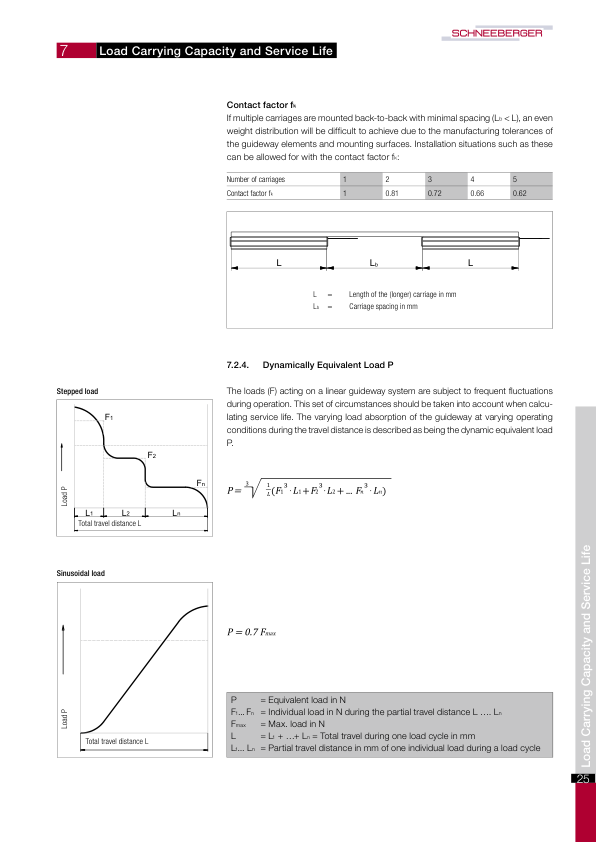
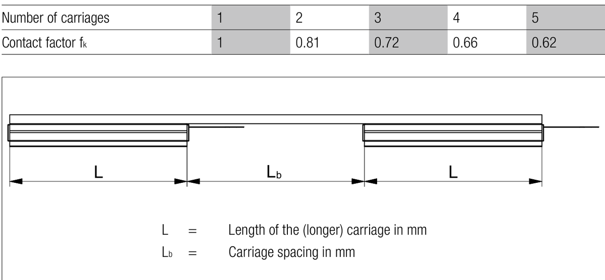
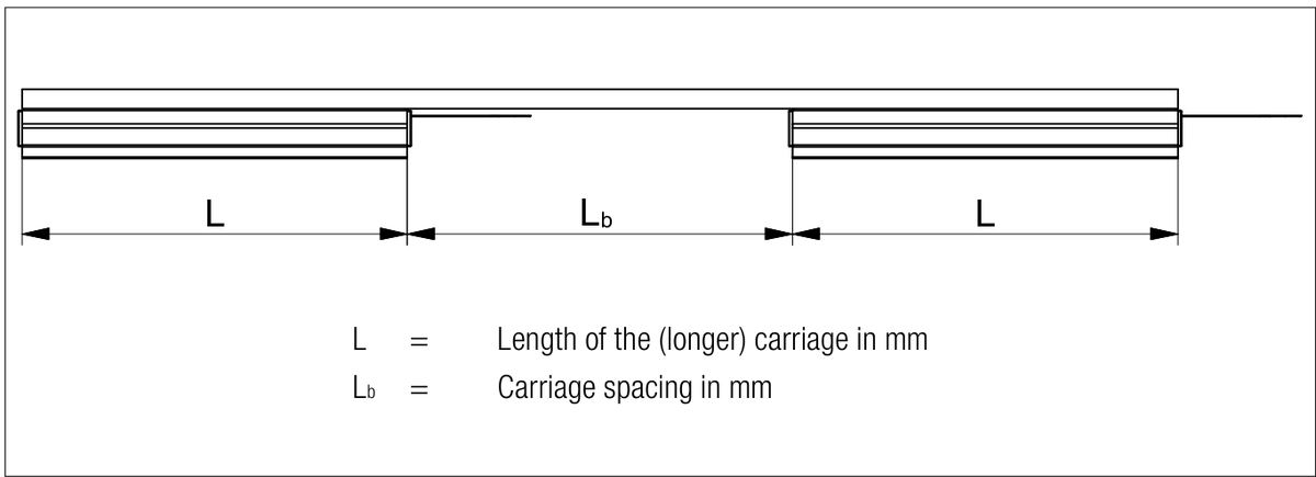
Contact factor fₖ
If multiple carriages are mounted back-to-back with minimal spacing (L_b < L), an even weight distribution will be difficult to achieve due to the manufacturing tolerances of the guideway elements and mounting surfaces. Installation situations such as these can be allowed for with the contact factor fk:
⚠️ 這可能不是一張表。有一種讀法認為這一頁沒有表格。請對照左邊的原頁確認;如果它不是表,按「排除」。
| Number of carriages | 1 | 2 | 3 | 4 | 5 |
| Contact factor fk | 1 | 0.81 | 0.72 | 0.66 | 0.62 |
7.2.4. Dynamically Equivalent Load P
The loads (F) acting on a linear guideway system are subject to frequent fluctuations during operation. This set of circumstances should be taken into account when calculating service life. The varying load absorption of the guideway at varying operating conditions during the travel distance is described as being the dynamic equivalent load P.
Stepped load
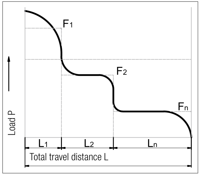
P = ∛((1/L)(F₁³ · L₁ + F₂³ · L₂ + ... Fₙ³ · Lₙ))
Load Carrying Capacity and Service Life
Sinusoidal load
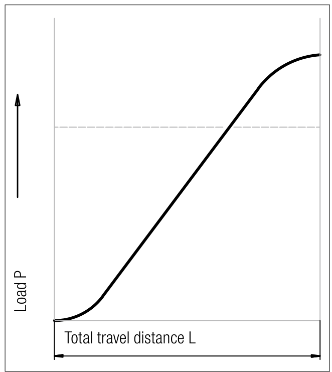
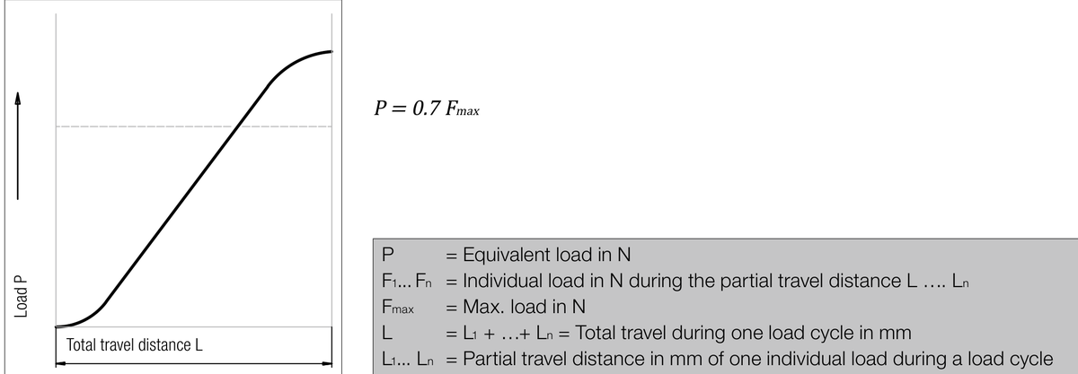
P = 0.7 Fmax
P = Equivalent load in N
F1... Fₙ = Individual load in N during the partial travel distance L ... Lₙ
Fmax = Max. load in N
L = L1 + ... + Lₙ = Total travel during one load cycle in mm
L1... Lₙ = Partial travel distance in mm of one individual load during a load cycle
25
L = Length of the (longer) carriage in mm
Lb = Carriage spacing in mm
SCHNEEBERGER

8
Ordering Information
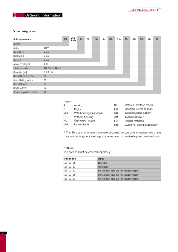
Order designation:
這張表定義了一組訂購代碼:100MSQ-Scale7-30.20-A-MG-0.1-RS-SB-SH-HA-KB —— 13 個區段
| Legend: | |||
|---|---|---|---|
| A | Analog | KI | Without Interface modul |
| D | Digital | RS | Special Reference mark |
| MG | With housing (Standard) | SB | Special Drilling pattern |
| OG | Without housing | SH | Special Stroke (1) |
| NL | Only circuit board | HA | Height-matched |
| MM | Micro Match | KB | Customer-specific lubrication |
(1) The SH option shortens the stroke according to customer's request and at the same time lengthens the cage to the maximum to enable highest possible loads.
Options:
The options must be ordered separately:
| Order number | Article |
|---|---|
| 556 100 151 | Base plate |
| 556 100 152 | Clamp plate |
| 556 100 160 | FFC extension cable 250 mm including Adapter |
| 556 100 161 | FFC extension cable 400 mm including Adapter |
| 556 100 162 | FFC extension cable 600 mm including Adapter |
26